Bundler calculation
To model a sequence in ipolog 4MF, both standard supply and standard bundler chains must be created and defined beforehand in the submodule 'Material flow planning > Edit standard process chain'. The single-variety standard supply process and the standard bundle chain are built separately for the time being and can be linked together in this submodule to obtain an overall standard process.
Log IDs that are subsequently assigned to a standard supply chain in the decision tree, which leads to a standard bundler chain, are then available in the submodule 'Material flow planning > Bundler editor'. Now concrete bundlers (a.k.a. sequences, baskets, car sets) can be formed here, log IDs assigned and further premises entered for calculation.
Structure of the submodule:
As shown in the screenshot, the standard supply chains, the bundler chains and the log IDs from the logistical quantity structure are listed there. In addition, the properties of the bundle chain can be defined.
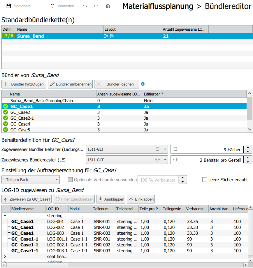
Creating a bundler:
By clicking on a bundler chain, it is selected and can be edited:
1.Container definition: Load carrier as well as bundler rack can be selected. Furthermore, the number of compartments as well as the number of containers per rack.
- Setting for order calculation:
- "One LOG ID per compartment": each compartment of a container is filled with exactly one LOG ID. With this option, no optional installation rate can be activated, as this can lead to a conflict of targets. The option "Empty compartments allowed" can be activated by hook. In this case, empty compartments are allowed in a box. If no parts are used in the corresponding bar, the compartment remains empty and is skipped. If the "Empty compartments allowed" function is deactivated, this means that every compartment in the box will be filled, even if a compartment is not used in every bar. Usecase: one Log ID per compartment corresponds to the use case for sequence-only bins, when consequently only one family of parts is in the bundler and the parts are in an "either/or" relationship. See examples 1 and 2 below.
- "x LOG IDs per bin": multiple LOG IDs can be filled per bin. The optional installation rate can be activated and adjusted. Initially 80% is set. Empty trays can also be (de)activated.
Usecase: This calculation logic "x LOG-IDs per compartment" corresponds to the principle "Car Set" or a shopping cart. So there are different part families in one bundler. See example 3 below.
-
Optional shoring rate: The optional shoring rate works like an additional factor that decides the frequency of parts consumption in the bundler beyond the summed shoring rate. See example 4.
-
Assignment of log IDs: The log IDs are displayed in groups. By clicking a single ID or with 'Ctrl' or 'Shift' several IDs can be marked and assigned to a bundler chain via the corresponding button. The bundle must be selected in the bundler overview and highlighted in blue.
Functionality of the underlying algorithm
The calculation of the bundlers is based on an algorithm that uses various values beyond the settings in the bundler editor. These are:
- Shoring rate (logistic quantity structure)
- Working times, break times (shift plan)
- Takt time (production data)
- Start/safety/reporting level in the process chain editor
- The settings in the bundler editor
The calculation of the sequencing is shown on the basis of different example cases. These differ by number of parts per compartment, empty compartments and the optional shoring rate.
Example 1 - general calculation logic
Bundler editor: One part per tray. No empty compartments allowed. Verbaurate: 100%. No optional shoring rate.
Process chain editor (For the corresponding bundler chain): Opening stock: 4; Reorder level: 2; Safety stock: 1.
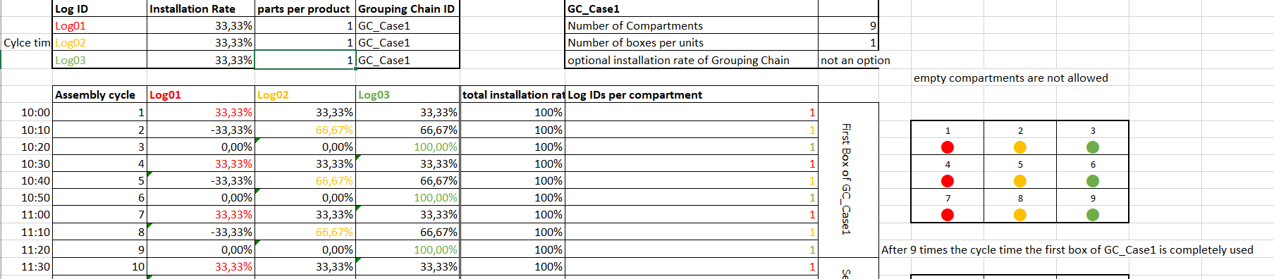
Log 1, Log 2 and Log 3 are to be bundled. All three parts have an installation rate of 33.33% or in words: these Log IDs are retrieved every third clock on average. The sum of the installation rate per clock is relevant for the calculation of the sequencing. In the example above, this takes ten minutes. In the first bar, the total usage rate is exactly 100% (33.33% (Log 1) + 33.33% (Log 2) + 33.33% (Log 3) = 100%), which means that one compartment/one Log ID is used up directly in the first bar. Here, the Log ID with the largest cumulative consumption rate (see next paragraph) is selected. In case of equality, the random principle decides. In the example above, Log 1 is placed in the bundler bin.
The next bar is calculated recursively. The logic is the same for all examples. In the following bar (10:10 in the example above), the initial shoring rate is added to the shoring rate of the previous bar. An exception is the log ID (or several log IDs, if applicable) that was consumed in the previous bar. For this cell, not only the initial usage rate (here 33.33%) is added, but 100% is subtracted due to the usage. For the second bar the following values result:
- Log 1: 33.33% (value from previous bar) - 100% (because of shoring) + 33.33% (initial shoring rate) = - 33.33%.
- Log 2: 33.33% (value from previous cycle) + 33.33% (initial shoring rate) = 66.67%.
- Log 3: 33,33% (value from previous cycle) + 33,33% (initial build rate) = 66,67%.
The next bar is calculated recursively again according to the principle shown above. However, Log 2 or Log 3 is used instead of Log 1 (selection is made randomly if the build rate is the same). In the example Log 2 is used. The calculation for bar 10:20 looks as follows:
- Log 1: -33.33% (value from previous bar) + 33.33% (initial build rate) = 0%.
- Log 2: 66.67% (value from previous pour) - 100% (due to shoring) + 33.33% (initial shoring rate) = 0%.
- Log 3: 66.67% (value from previous cycle) + 33.33% (initial shoring rate) = 100%.
In the example given, a box with 9 compartments was selected. Accordingly, the first box is completely consumed after nine cycles. The initial stock on the line is four boxes, the reorder point and safety stock are two and one boxes respectively. In addition, the number of boxes per rack was defined as "2".
- Earliest staging time: In the 18th cycle. This means in the cycle in which the second box will be completely consumed.
- Latest staging time: After the 27th cycle. Three boxes have been used up and the last box on the line is broken into. The safety stock level is fallen short of, resulting in the latest staging time.
Example 2 - empty boxes
Differences of the configuration compared to example 1: The Log IDs have different installation rates (Log 4: 30%; Log 5: 20%; Log 6: 10%). Since the total is <100%, this does not necessarily result in consumption in every cycle. In the "Case 2 and 3" spreadsheet, none are allowed; in "Case 2-1 and 3.1", empty compartments are allowed in the bundler bin.
The calculation logic for sequencing is analogous to Example 1. The differences are discussed below, due to the differences in configuration.
For both cases, the total shoring rate in the first cycle is 60%, so no shoring takes place. The 100% mark is not reached until the second cycle and the Log ID is installed. If no empty compartments are allowed (Case 2 and 3), the Log ID is placed in the first compartment of the first box. If empty boxes are allowed (Case 2-1 and 3-1), the first box is left empty and the second box is filled.
Example 3 - x Log IDs per compartment
Configuration: "x LOG IDs per compartment".
The calculation logic for sequencing is analogous to example 1. As soon as the sum of the obstruction rate is >=100%, a Log ID is consumed. If the sum of the shoring rate is >=200%, two Log IDs are consumed and placed in the bundler bin. If >= 300%, three Log IDs are consumed and so on. In the example "Case 4" this situation occurs in the second cycle. The shoring rate is 240%, so two Log IDs are consumed. Therefore, Log 11 and Log 12 are consumed.
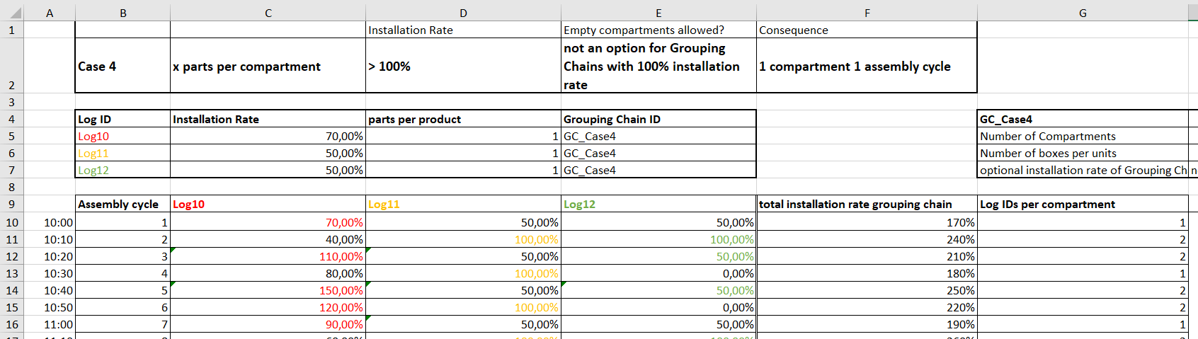
Note: Since the sum of the installation rate of the log IDs is always >100% here, no empty compartment can occur in the bundler container. Each cycle consumes one compartment of a bundler bin.
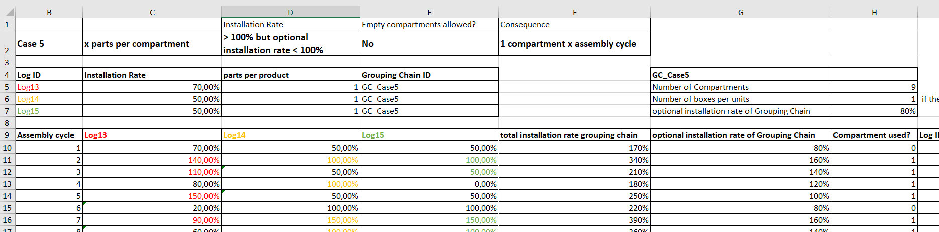
Example 4 - optional shoring rate
In the previous examples, the total obstruction rate was always used as a criterion for the consumption of logs in the bundler. Now, the optional obstruction rate is added and forms the primary decision criterion that determines the consumption of Log IDs.
In the example shown, in addition to the Log IDs (Log 13: 70.00%; Log14: 50.00%; Log15: 50.00%)
an opt. usage rate of 80% is assumed. In the first bar, this results in a total obstruction rate of 70% + 50% + 50% = 170% and a (set) optional obstruction rate of 80%. Up to now, the total shoring rate of 170% would have triggered the shoring of exactly one Log ID. The added optional shoring rate is 80% and thus below 100%. In this case, no shoring is triggered, the compartment remains empty or is filled in the following cycle (depending on the activation of the "allow empty compartments" criterion).
The subsequent, second takt is calculated analogously to example 1. This results in a total shoring rate of 340% and an optional shoring rate of 80% (optional shoring rate takt 1) + 80% (optional shoring rate takt 2) = 160%. As the 100% mark is exceeded, a consumption is triggered. In this context, however, the optional shoring rate only indicates the fact that shoring takes place, but it does not determine the quantity. The quantity is still determined by the total usage rate, which is 340% in this case. This means that three Log IDs are installed, in this example all three Log IDs.
For the third bar, the calculation of the optional build rate is similar to the already known recursive pattern:
Opt. bonding rate (bar 3) = opt. bonding rate (bar 2) - 100% (since logs were consumed in this bar) + 80% initial opt. bonding rate = 160% - 100% + 80% = 140%. Also in this takt the opt. build rate is > 100% and parts are consumed in the bundler.
The calculation of the sum of the shoring rate or the total shoring rate follows the pattern presented in example 1.