Introduction
On this page we explain in detail the calculation methods for order and transport calculation for direct and route transports.
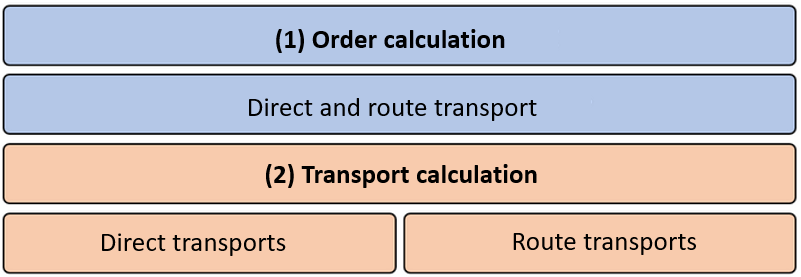
(1) Order calculation
Order calculation - General
A transfer order is created when parts consumption reaches or falls below defined stock values.
The order calculation for direct and route transports uses the same calculation logic on the one hand for the full load and on the other hand for the empties process.
Storage parameters
Based on the staging requirements (consumption times) and the storage parameters from the supply and disposal chains, the earliest and latest possible staging times (FBZ and SBZ) can be calculated for each part.
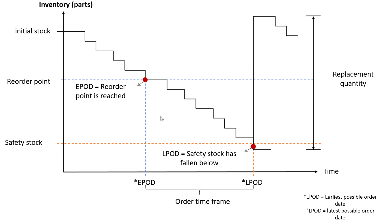
Full stock
- Opening stock
- Reorder level
- Safety stock
- Replenishment quantity
1. opening stock
- The opening stock serves as the simulation and calculation start of the transfer orders.
2. reorder point
- The earliest possible staging point (EP) is the point in time at which the reorder level is reached.
- The reorder point therefore indicates that there is free storage space available at the staging location and that the replenishment quantity can be delivered as replenishment.
- The reorder level must not be lower than the safety stock level.
- Reorder level could also be described as "stock at earliest staging point".
3. Safety stock level
- The latest possible provision time (SBC) is the time at which the safety stock level has fallen below the safety stock level.
- The safety stock level must not be higher than the reorder level.
4. replenishment quantity
- The replenishment quantity describes the replenishment quantity in load carriers or loading units.
- The stock increases at the time of fulfillment of a transfer order by the number of replenished parts (the replenishment quantity is multiplied by the load carrier or load unit content and thus converted into the number of parts).
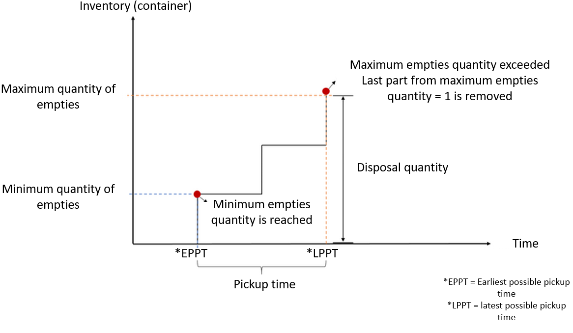
Empties
1. minimum quantity of empties
- The minimum empties quantity indicates the stock of empty containers from which the empties can be removed at the earliest.
- The earliest possible collection time (EPOD) is the time at which the minimum empties quantity is reached.
2. maximum quantity of empties
- The maximum empties quantity indicates the stock of empty containers at which the empties must be removed at the latest.
- The latest possible collection time (LPOD) is the time at which the maximum empties quantity has been exceeded.
3. marking the order as a "push order".
- in the past, we used to convert the earliest/latest pickup time to the earliest/latest staging time, because at that time the transport calculation was only able to calculate earliest staging times. Now we mark the orders as "push orders", which means that the selected times are relevant for the pickup of the material, not for the delivery. Nevertheless, the label "earliest/latest staging time" is still currently used for lack of a better term, which has been supplemented with the declaration as push/pull principle
Preconditions for valid orders
- A logistics quantity structure has been imported and saved
- Staging requests have been created or imported and saved
- A layout is imported and saved
- A route network is created, breakpoints defined and areas from the layout assigned
- At least one standard supply chain is created and saved
- Imported parts from the LMG are assigned to a standard supply chain via the decision tree
- Supply and disposal chains are completely defined including storage parameters
Order calculation full goods - last stage (pull principle).
EPPT= Time at which the reorder level is reached.
LPPT = time at which the reorder level falls below the safety stock level.
Notice:
By importing or generating provision requests, concrete consumption times for the last stage are known, so that a concrete provision window (FBZ-SBZ) in which the order must be fulfilled can be calculated on the basis of the initial, reorder and safety stock levels.
Order calculation for full products - previous stages (pull principle)
For all stages before the last stage, no concrete consumption times are yet known. Therefore, an approximate consumption time is calculated. This results from the following input data:
- EPPT (stage n)
- LPPT (stage n)
- Discharge time at the sink
- Driving from source to sink
- Loading time at the source
Calculation
Assuming permanent operation, the calculation is as follows:
assimilated replenishment time (level n) = 1/2*(FBZ(level n) + SBZ(level n))
total transport time: unloading time + travel time + loading time
Consumption time (level n-1) = assimilated replenishment time - total transport time
The calculation of the earliest and latest staging time (EPPT and LPPT) is analogous to the order calculation full load - last stage (pull principle).
EPPT = Time at which the reorder point is reached.
LPPT = time at which the safety stock level is fallen short of.
Notice:
Route transports currently use an average travel time of eight minutes plus the loading and unloading time for the selected material.
Consideration of the shift schedule for the calculation of the assimilated replenishment time:
The calculation of the assimilated replenishment time is based on the production shift schedule. Assuming an order has EPPT= 10:00 and LPPT = 12:30 and a half-hour break is scheduled between 11:45 and 12:15, the result for the assimilated replenishment lead time is not 11:15, but a shift forward by 15 minutes to 11:00 due to the break.
Consideration of the shift schedule for the calculation of the consumption time:
The consumption time (level n-1), since it is a logistics process, is independent of the production shift schedule, but it depends on the shift schedule of the means of transport selected for this transport. This means: If the total transport time is 10 minutes, the assimilated replenishment time is calculated to 12:20 and we have a half-hour break from 11:45 to 12:15, the consumption time (level n-1) is set to 11:40.
Order calculation empties - single stage (push principle)
In contrast to the order calculation of the full product, the sawtooth curve does not run downwards through the parts consumption, but upwards and is counted up in container units.
EPPT = Time at which the minimum empties quantity is reached.
LPPT = Time at which the maximum empties quantity is exceeded.
Remark:
For calculation purposes, the LPPT corresponds to the time at which the last part is removed from the nmax+1 container (nmax = maximum empties quantity).
Order calculation empties - multi-stage (push principle)
In the multi-stage empties process, the actual staging times for the stages between the first source and the last sink are still unknown. Therefore, an approximate staging time is calculated. This results from the following input data:
- EPPT (stage n)
- LPPT (stage n)
- Discharge time at the sink
- Travel from source to sink
- Loading time at the source
Provision time for stage n+1 = 1/2*(FBZ(stage n) + SBZ(stage n)) + unloading time + driving time + loading time
EPPT = Time at which the minimum quantity of empties is reached.
LPPT = Time at which the maximum empties quantity is exceeded.
Order calculation empties - full/empty exchange
The full/empty exchange can take place between a stage of the full and first stage of the empty process. This setting can be selected in the view of the disposal chains.
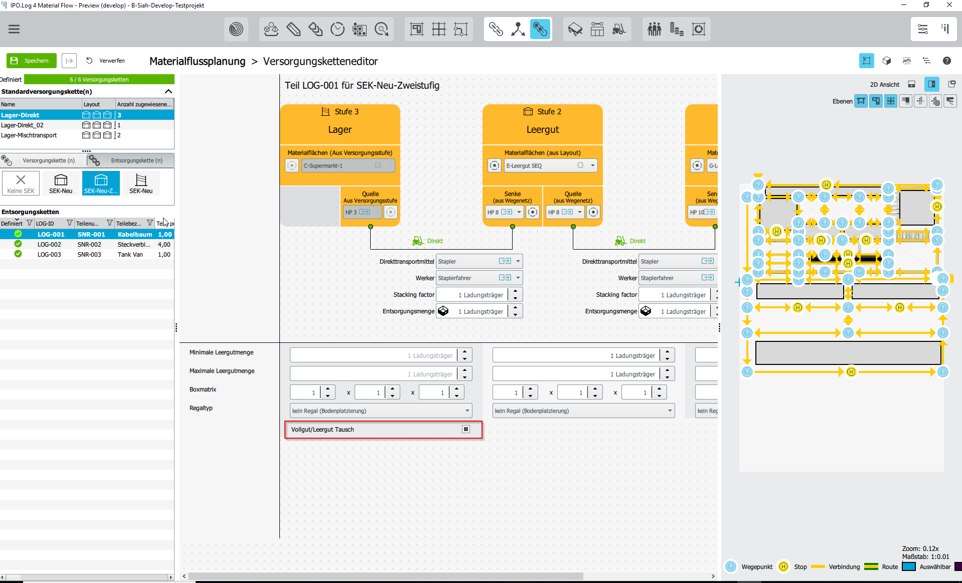
Notes:
- The checkbox for the full/empty container exchange is only visible if the same means of transport type is selected for supply and disposal.
- Empties that are transported on the basis of a full/empty exchange do not receive their own order in the order list. In terms of time, this empties order is executed directly after the respective full container order.
- The handling times (loading and unloading empties) are taken into account in the transport calculation.
- In the column "Order with full/empties swap" in the order list, this is marked with an "x" in the full goods order.
Reasons for unfulfillable orders
More information here: Solution for unfulfillable orders
- No shift plan is assigned to a means of transport type
- No worker type assigned
- Process time exceeds maximum tour duration (clocked tours)
- No suitable takt (clocked tours)
- Average speed of the means of transport is 0
- No means of transport type assigned
- Breakpoint of the source differs from the breakpoint of the route start
- Breakpoint of the source is missing
- Breakpoint of the sink is missing
- No valid breakpoints set
- No suitable shift
- A single order alone overloads an entire tour
- No trailer type defined
- No route to the sink found
- No destination sink found
(2) Transport calculation
Transport calculation - General
Basis for the transport calculation are calculated, fulfillable orders from the order list.
Transport calculation target and restrictions:
Objective function: Minimize transportation demand
under the following constraints:
- Delivery time window (FBZ-SBZ)
- Shift schedule (working and break times)
- Capacities
1. Direct transports: stacking factor
2. Route transports: chaining factor tractor type + max. loading weight + max. area utilization + trailer areas (resource management)
4. Route network/route
The following simulation parameters have further influence on the transport calculation:
- Granularity of the transport calculation - calculate resource requirements fine or coarse.
- Route finding strategy - shortest transportation time or shortest transportation route
- Transfers during breaks
- Use of weight restrictions for transports
A detailed description of the simulation parameters can be found here
Transport calculation - direct transports
Input:
A list L of transport orders for a direct transport type sorted in descending order by average staging time. (late -> early)
Route network with waypoints, stops and restrictions.
Direct transport means, especially average speed, assigned worker type (including distribution time) and shift schedule.
Transport simulation parameters
Transport groups
Output:
A list R of direct transport instances D that refer to a list T of transports.
Algorithm:
- For each means of transport type + worker + transport group combination, the minimum number of means of transport required is calculated. Minimum means the pure process time, disregarding empty runs or standing times. Thus, the sum of all processes to be performed is taken and added up, divided by the total net working time, and rounded up to the sum x. The number of means of transport is then calculated. For this number, means of transport instances are initialized with the first orders of the descending sorted list as late as possible.
- As long as L is not empty
- Check if there is an order A which in combination with the last fulfilled order A' results in a seamless combination (cf. condition 1) (i.e. HP sink of the first order corresponds to the HP source of the following order). If so, take it out of L and add A to T. Otherwise, take the first order A from L and find the best matching transport from T to add A to T.
- If A violates capacity limits, shift schedules or delivery time windows, note error condition for A.
- For each direct means of transport instance D of the required direct means of transport type and the required transport group G in R
- Condition1: If D is able to append A seamlessly (without pause) and without empty run to a transport in front (transport calculation strategy late) or behind (transport calculation strategy early):
- Add A to the list of orders T transported by D in such a way that the transports can be executed seamlessly.
- Start a new run of the outer loop
- If D is able to append A seamlessly (without pause) but with empty run to a transport in front (transport calculation strategy late) or behind (transport calculation strategy early):
- add A to the list of orders T transported by D in such a way that the transports can be executed seamlessly
- Start a new run of the outer loop
If D is able to append A with a pause to a tour in front (transport calculation strategy late) or in the back (transport calculation strategy early) but without an empty run: - Add A to the list of orders T transported by D in such a way that the transport takes place as early/late as possible, depending on the transport calculation strategy.
- Start a new run of the outer loop
- If D is able to append A with a break to a tour at the front (transport calculation strategy late) or at the back (transport calculation strategy early) with an empty run:
- Add A to the list of orders T transported by D in such a way that the transport takes place as early/late as possible, depending on the transport calculation strategy.
- Start a new run of the outer loop
- Add new direct transport instance D to R, initialize T(D) with A such that A satisfies the transport calculation strategy (early/late).
Sequence of test conditions (prioritization rules):
- without pause (standstill/unproductive time) and without empty run
- without pause with empty run
- with pause without empty run
- with pause with empty run (transport possible with this means of transport instance?)
Transport calculation - route transports
The route calculation consists of two successive phases. In phase (1), order collection, orders that can be fulfilled on a tour are collected together without the exact start or end time already being fixed. In phase (2), scheduling, a start time is fixed for each tour in such a way that the number of required route train instances is minimized. Phase 2 is very analogous to the direct transport calculation for dynamic tours.
Pseudo code route transports
(1) Order collection
Input:
A list L of transfer orders for a route ordered by earliest staging time.
Route history with distances between waypoints to calculate travel times
The route train configuration (tractor with maximum speed, chaining factors)
Output:
A list R of routes
Algorithm:
- As long as L is not empty
- Create an empty tour T
- Take first order A from L and add A to T
- If T violates capacity limits, shift schedules or delivery time windows, note error condition for A
- For each order A in L
- If A can be added to T without violating capacity limits, shift schedules or delivery time windows
- Add A to T
- Remove A from L
- Add T to R
This algorithm is optimized by a series of early terminations.
(2) Termination
Input
A list F of tours, with the earliest and latest possible start times, so that no shift schedules or delivery time windows are violated. F is ordered by earliest possible start time.
Output
A start time S_T for each tour T in F
A routing instance R_T for each tour T in F
A list B of required routing instances
Algorithm
- Initialize B to empty list
- For each tour T in F
- For each routing instance R in B
- If R is able to connect T seamlessly to another tour:
- R_T = R
- S_T = end time of the previous tour
- Start new run of the outer loop
- For each routing instance R in B
- If R is able to connect T to another tour with a pause:
- R_T = R
- S_T = earliest possible start time of T
- Start new run of the outer loop
- Add new routing instance R to B
- R_T = B
- S_T = earliest possible start time of T